Abstract
Sections
Setup
I knew from the onset that I wanted just one component which, once attached to a Game Object, would create and provide control over a vast ocean surface as well as the underwater post processing effects. To see how I might cut out that Mesh Renderer middleman, I looked at Unity's own Water System built for the High Definition Render Pipeline (HDRP). HDRP splits the water system into a frontend component, and a large backend which handles all of the rendering processes. This allows much computation to be shared between water surfaces and precludes post processing from ever stacking. The crux of the HDRP system is a command buffer provided by the Render Pipeline and executed every frame.
Command buffers are essentially a sequence of rendering instructions which you create and then send off to the GPU. They can then be executed again and again without having to re-send the instruction, among other performance benefits.
Since I am using the Universal Render Pipeline, I hook into the per-camera rendering callback like so:
RenderPipelineManager.beginCameraRendering += RenderSurface;void RenderSurface(ScriptableRenderContext context, Camera camera)
{
CommandBuffer commandBuffer = CommandBufferPool.Get("Water CMD");
UpdateSurface(waterSurface, commandBuffer, context, camera);
context.ExecuteCommandBuffer(commandBuffer);
context.Submit();
commandBuffer.Clear();
CommandBufferPool.Release(commandBuffer);
}Wave Displacement
You might have heard of the Fast Fourier Transform before, it has been used in dozens of games and movies after it was proposed in the 2004 paper Simulating Ocean Water by Jerry Tessendorf.
I learned of it from a source I am much more familiar with; a 2023 Youtube video by Acerola, a graphics programmer entertainer; I Tried Simulating The Entire Ocean.
What must be understood before understanding the Fourier Transform is that any periodic waveform can be identically reproduced with a sum of sinusoids.
The purpose of Fourier Transform, then, is to take a waveform and decompose it into that sum of sinusoids.
The output is now in the "frequency domain" which, as opposed to describing how amplitude at a given time (time domain), describes the amplitude of a wave at a given frequency.
For example, for a wave of frequency 30hz we see a spike in the frequency domain at 30hz.
The size of the spike is proportional to it's amplitude, as we see in the figure below.
These wave spectra can generate tens of thousands of frequencies, at a resolution of 256x256, we need to perform the IFT over 65,000 times.
This is the 'fast' part of the Fast Fourier Transform.
The FFT uses a 'Butterfly Algorithm' to recursively split the input data in half which avoids unnecessary calculations.
Please see here for a more in-depth exploration of the FFT.
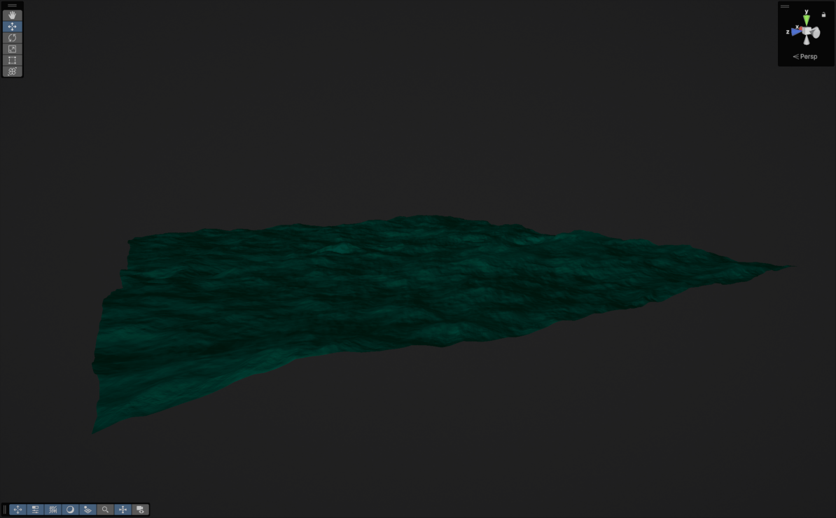
To summarise all of this in a sentence: we generate and progress a frequency domain wave spectrum, then perform the Inverse FFT over all the texture points to attain an amplitude map in the time domain.
From the amplitude map, slope and displacement maps are derived (including vertical and horizontal offsets), these the textures we will send to the ocean shader:
However, even with very detailed wave spectra, we have not completely eradicated the tiling issue. It is inevitable that any periodic waveform, or sum or periodic waveforms, will repeat given enough distance. However, the FFT is so fast we can actually compute several wave spectra simultaneously and scale them over the ocean surface. The literal millions of waves all interact and distort one another virtually eradicating tiling up to an extreme distance.
As one last trick I learned from HDRP, you can define constants as part of a compute shader's kernals. I used to this give the user control over the resolution of the wave spectra and subsequent FFT passes as a graphics option.
#pragma kernel RowPass_128    FFTPass=RowPass_128                 FFT_RESOLUTION=128    BUTTERFLY_COUNT=7
#pragma kernel ColPass_128    FFTPass=ColPass_128   COLUMN_PASS   FFT_RESOLUTION=128    BUTTERFLY_COUNT=7
#pragma kernel RowPass_256    FFTPass=RowPass_256                 FFT_RESOLUTION=256    BUTTERFLY_COUNT=8
#pragma kernel ColPass_256    FFTPass=ColPass_256   COLUMN_PASS   FFT_RESOLUTION=256    BUTTERFLY_COUNT=8
#pragma kernel RowPass_512    FFTPass=RowPass_512                 FFT_RESOLUTION=512    BUTTERFLY_COUNT=9
#pragma kernel ColPass_512    FFTPass=ColPass_512   COLUMN_PASS   FFT_RESOLUTION=512    BUTTERFLY_COUNT=9

[numthreads(FFT_RESOLUTION, 1, 1)]
void FFTPass(uint3 id : SV_DISPATCHTHREADID)
{
    for (int i = 0; i < 8; i++)
    {
        #ifdef COLUMN_PASS
            _FFTTarget[uint3(id.xy, i)] = FFT(id.x, _FFTTarget[uint3(id.xy, i)]);
        #else
            _FFTTarget[uint3(id.yx, i)] = FFT(id.x, _FFTTarget[uint3(id.yx, i)]);
        #endif
    }
}
Water Shading
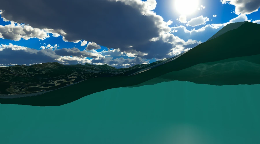
For any given ray of light hitting the ocean surface, we see that several things can happen. It may reflected off the surface into the camera, resulting in a mirror reflection of the sky above. Or it may penetrate the ocean surface and then be scattered back out. Since red wavelengths more likely to be absorbed than scattered, we observe that areas of higher scattering the water appears lighter and more blue. For any given fragment, we determine an approximation of how light interacts with the surface using a BRDF function.
In the GDC talk on Atlas mentioned above, see here, the developers present a Microfacet BRDF model, which consists of a Fresnel reflectance term, a normal distribution function and a masking function.
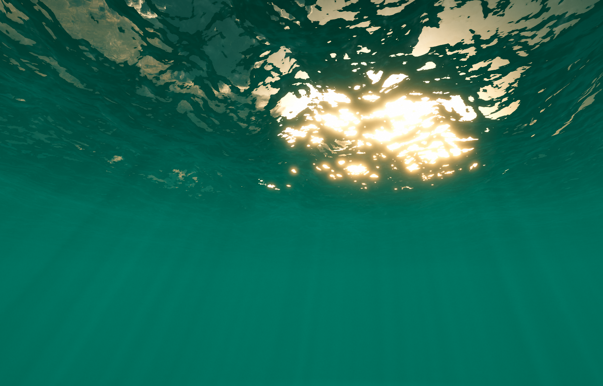
The Fresnel reflectance term describes areas where we will see scattered light vs reflected light, as well as specular highlights. It can be computed using the indices of refraction of air and water which, when viewed from under the surface, creates an effect called Snell's window. This describes how light exiting the ocean volume at a harsh angle totally internally refracted leading to a window above the camera where the sky can be seen, surrounded by an "opaque" surface.
The normal distribution function describes which direction relative to the normal vector of the surface incoming light is likely to reflect in.
And finally the masking term, or Geometric Attenuation term, the object self-shadowing as you view it at an increasingly perpendicular angle.
Finally, the developers use several "fudge terms" to mimic the likelihood of observing scattered light rays at any given part of the ocean:
- An ambient term, we observe that some light is scattered uniformly.
- A height term, we observe that more light is scattered in wave peaks.
- A view term, we observe that we are more likely to see scattered light if the surface normal coincides with the view direction.
- A shadow term, we observe that we are more likely to see scattered light if the surface normal coincides with the light direction.
Dynamic Detail
- Dynamic Meshing
- Vertex Tessellation
Dynamic meshing is how I am refering to constructing the mesh data that will be sent to the GPU.
Like using Levels of Detail to render decimated versions of objects as they get further from the camera, the same can be done to oceans only a little more complicated.
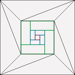
Upon creating a HDRP ocean, three meshes are generated; a dense central grid, a rectangular grid mesh and a colossal outer mesh which is essentially a flat plane with a hole in it.
These meshes are dynamically scaled and rotated to fill the surface.
Put together, the meshes look like this:
A neat optimisation here is to use indirect GPU instancing to draw the ring meshes since they are drawn dozens of times.
This eliminates duplicate vertex batches by asking the GPU to cache the ring mesh and simply reuse it when requested.
We fetch get the instance ID in the vertex shader (before tessellation) and apply rotation and scaling data from a Structured Buffer prepared beforehand.
These meshes are frustum culled when generating the buffer, and again in the tessellation stage (per mesh then per triangle).
Secondly, we use GPU Vertex Tessellation to generate more vertices on the GPU.
In a tessellation shader, the distance from the vertex to the camera is used to generate a tessellation constant.
This is used to recursively subdivide the ocean mesh, creating more displaceable geometry without sending it to the GPU with the rest of the scene.
Underwater Rendering
One idea was to calculate the height at a given position from the displacement maps. However, this does not account for the horizontal component of the FFT's, or the shape of the water mesh.
So I tried to recapture the height of the surface mesh after it is rendered using a separate, orthographic camera above the view camera. Although multiple camera's does effect performance, this created the effect I wanted for a small area around the player. However, later in this project I introduced water cutouts, areas where the water would be hidden such as the inside of a submarine. This solution was unable to account for the myriad of complex ways a glass window could intersect the water surface.
My most recent attempt involves generating two masks; a position mask and a surface face mask.
The face mask is captured to a render texture in a pre-pass, which renders the ocean surface before anything else using it's own depth texture. Front/back face information is stored in the red channel; front as 1.0, back as 0.5, leaving 0 where there is no surface present. To do this, I reused the pre-pass I had already implemented to capture the surface depth, which is useful for several underwater effects.
The position mask is computed using the position of the water surface and a position computed at the maximum depth from the camera using the screen space uv coordinates.
With these two masks, I can test if a given fragment is underwater with this slightly strange logic:
bool ShouldRender(float2 uv, float sceneDepth)
{
    float surfaceMask = SAMPLE_TEXTURE2D(_SurfaceFaceMask, sampler_PointClamp, uv).r;

    if (surfaceMask > 0.9)
        return false;

    float3 skyboxPos = ComputeWorldSpacePosition(uv, 0.00001, UNITY_MATRIX_I_VP); // Tiny epsilon to remove line artefact created just under water plane.
    return surfaceMask > 0 || (_SurfacePosition.y > skyboxPos.y);
}Using backfaces in this way does create a small issue where extremely violent FFT waves can roll in on themselves creating backfaces above the water surface. These artefacts are generally small and could be removed in a compute shader. The last approach I have considered is using some sort of vertical smearing to propagate the lowest water surface pixels on the screen downwards. This would be performed in a compute shader after the depth pre-pass has been rasterized, and combined with the position mask would create a perfect waterline, so I may revisit this section later.
Finally with that done, I simply tint the screen with an underwater absorption color using the combined water and scene depth.
Caustics
Many games achieve this by simply mapping a precomputed, animated texture to underwater geometry. This is a quick and dirty approach which is very effective for many games, especially those where the ocean waves are constant or performance is a large concern. However, it is possible to generate caustic patterns in real-time that actually reflect the state of the ocean surface, whether calm and slow or violent and stormy.
This article by Evan Wallace describes how this can be done by constructing a dense 'virtual plane' and refracting the vertices as if travelling through water. The new and old vertex positions are then ran through a ray, plane intersection function and given to the fragment shader. The color of each fragment is then determined by the difference in area between the non-refracted plane and the refracted one, taking advantage of the fact that fragments are computed in sets of four. In Unity that looks like this:
float Frag (Varyings i) : SV_Target
{
    float intialTriangleArea = length(ddx(i.originalPos)) * length(ddy(i.originalPos));
    float refractedTriangleArea = length(ddx(i.refractedPos)) * length(ddy(i.refractedPos));

    return intialTriangleArea / refractedTriangleArea;
}
Godrays
float SampleGodrays(float3 positionWS, float3 lightDirection)
{
    float3 normal = float3(0.0, -1.0, 0.0);

    // Project caustics texture in light direction.
    float3 forward = refract(lightDirection, normal, 1.0 / _IndexOfRefraction);
    float3 tangent = normalize(cross(forward, float3(0.0, 1.0, 0.0)));
    float3 bitangent = cross(tangent, forward);

    float3 sampleCoord = positionWS * _TilingFactor;
    float2 uv = float2(dot(sampleCoord, tangent), dot(sampleCoord, bitangent)) * 0.5 + 0.5;

    // Sample caustics texture at a low LOD of for some free blurring.
    // This means we can get away with a larger step size because the artefacts are naturally hidden.
    return SAMPLE_TEXTURE2D_LOD(_CausticsTexture, sampler_LinearRepeat, uv, 5).r;
}
Water Cutouts
An SDF essentially allows you to work out how far a given point is from the surface of a user defined shape. The distance is negative when the point is within the shape, and positive when it is outside. To produce an SDF that closely matches the hull of my submarine, I wrote a custom SDF generator which converts a mesh to a 3D texture where the red channel contains the distance from the surface. The generation algorithm first evaluates the bounds of the mesh, and then creates a texture with a user defined resolution to fit those bounds. Then, for each point in the 3D texture, the distance to every triangle in the mesh is evaluated and a value is updated every time a smaller distance is found.
This is performed within a compute shader, and looks like this:
float EvaluateTriangle(int triangleIndex, float3 pos)
{
    // a, b and c are the vertices of the triangle.
    float3 a = _Vertices[_Triangles[0 + triangleIndex * 3]];
    float3 b = _Vertices[_Triangles[1 + triangleIndex * 3]];
    float3 c = _Vertices[_Triangles[2 + triangleIndex * 3]];

    float3 pointOnTriangle = ClosestPointOnTriangle(pos, a, b, c);
    float3 normal = cross(b - a, c - a);

    float3 v = pos - pointOnTriangle;
    float3 dirToFace = normalize(v);
    float distToFace = length(v);

    if (dot(dirToFace, normal) < 0)
    {
        distToFace *= -1;
    }

    return distToFace;
}

float SmallestPointDistanceToMesh(float3 pos)
{
    float minAbsoluteDistance = 3.40282347e+38F;
    float minDistance = 3.40282347e+38F;

    for (int i = 0; i < _NumTriangles; i++)
    {
        float distance = EvaluateTriangle(i, pos);
        float absoluteDistance = abs(distance);

        if (absoluteDistance < minAbsoluteDistance)
        {
            minAbsoluteDistance = absoluteDistance;
            minDistance = distance;
        }
    }

    return minDistance;
}Once the SDFs have been produced, they are sent to the GPU as a sort of dictionary. Then, any submarines simply have to register an ID and transformation matrix to cut out any water within the SDF. This is done by calculating the world space position of the water surface (and the raymarching function) and multiplying it by the world to local matrix provided. Finally the position is converted to uv coordinates and evaluated against the pre-cached dictionary.
To avoid sampling the SDF's for every fragment, I also implemented a bounding box check which must be passed before sampling the SDF texture. Cutout instances are also frustum culled to avoid checking against out-of-view cutouts.
Sources
The Fourier Transform
https://www.thefouriertransform.com/Wakes, Explosions and Lighting: Interactive Water Simulation in Atlas
https://www.youtube.com/watch?v=Dqld965-Vv0Reflection, Refraction and Fresnel
https://www.scratchapixel.com/lessons/3d-basic-rendering/introduction-to-shading/reflection-refraction-fresnel.htmlOcean Simulation - antoniospg
https://antoniospg.github.io/UnityOcean/OceanSimulation.htmlSimulating Ocean Water - Jerry Tessendorf
https://people.computing.clemson.edu/~jtessen/reports/papers_files/coursenotes2004.pdfI Tried Simulating The Entire Ocean - Acerola
https://www.youtube.com/watch?v=yPfagLeUa7kCrash Course in BRDF Implementation - Jakub Boksansky
https://boksajak.github.io/files/CrashCourseBRDF.pdfRendering Realtime Caustics in WebGL - Even Wallace
https://medium.com/@evanwallace/rendering-realtime-caustics-in-webgl-2a99a29a0b2cPeriodic Caustic Textures
https://www.dgp.toronto.edu/public_user/stam/reality/Research/PeriodicCaustics/index.html